Can High Attenuation Cause Disruption
What’s the Difference Between Signal Attenuation and Disruption?
In conversations about fiber optic performance, two terms often surface interchangeably: attenuation and disruption. To the untrained ear, they might sound like synonyms—both suggest something’s gone wrong with the signal. But in reality, they describe fundamentally different phenomena, operating on different scales, with distinct causes, implications, and remedies.
Understanding this distinction isn’t just academic—it’s essential for diagnosing network issues, designing resilient infrastructure, and avoiding costly missteps. So let’s clarify: what really separates attenuation from disruption? And why does it matter to engineers, operators, and planners alike?
Isn’t Signal Loss Just Signal Loss? Why Split Hairs?
Because not all signal degradation is created equal—and conflating the two can lead to wrong conclusions and wasted effort.
Attenuation is the gradual, predictable reduction in optical power as light travels through fiber. It’s a continuous, physical property of the medium—like friction slowing a rolling ball. Even in a perfect, brand-new fiber under ideal conditions, attenuation exists. It’s measured in decibels per kilometer (dB/km) and is governed by the laws of physics: Rayleigh scattering, material absorption, and waveguide imperfections.
Disruption, by contrast, refers to an abrupt, often localized event that interrupts, distorts, or corrupts the signal path—sometimes catastrophically. Think of it as a pothole or roadblock on that same highway: not a gentle slope, but a sudden break in continuity. Disruption may cause total loss of signal (a “dark fiber”), intermittent errors, or data corruption—even if overall attenuation appears normal.
In short:
- Attenuation = expected, quantifiable weakening
- Disruption = unexpected, often pathological failure
One is managed through link budgeting; the other demands fault isolation and remediation.
Is Attenuation Always a Problem—or Just Part of How Fiber Works?
Attenuation is inherent, not defective. In fact, modern single-mode fiber is engineered to minimize it to astonishing levels:
- ~0.35 dB/km at 1310 nm
- ~0.20 dB/km at 1550 nm
- As low as 0.15 dB/km in ultra-low-loss fibers
This means a signal can travel 100 km and still retain ~1% of its original power—enough for sensitive receivers to decode. Engineers account for this in the optical link budget, which includes:
- Fiber attenuation
- Connector and splice losses
- System margin (for aging, temperature, etc.)
As long as total loss stays within the transceiver’s power budget (e.g., -28 dBm to -3 dBm for 10G-LR), the link functions flawlessly. In this sense, attenuation isn’t a “problem”—it’s a design parameter.
The real issue arises when attenuation exceeds expectations—due to poor splices, tight bends, or aging. But even then, it’s usually a matter of degree, not kind.
So What Exactly Counts as a “Disruption”?
Disruption implies a break in signal integrity that isn’t explained by gradual loss alone. It can manifest in several ways:
1. Complete Signal Loss (Fiber Cut or Break)
A backhoe severing a conduit, a rodent chewing through a drop cable, or a connector pulled loose—these cause infinite attenuation (i.e., no light reaches the receiver). This is pure disruption: binary, total, and urgent.
2. Intermittent or Transient Errors
A loose connector that wiggles with temperature changes, a microbend that appears only under wind load, or a contaminated interface that degrades under high humidity—these cause flapping links or rising bit error rates (BER) without a steady increase in loss. The signal isn’t just weak; it’s unreliable.
3. Signal Distortion Without Power Loss
Here’s where it gets subtle. In high-speed coherent systems, you can have near-perfect received power but still suffer massive errors due to:
- Polarization-mode dispersion (PMD)
- Chromatic dispersion exceeding compensation limits
- Nonlinear effects like four-wave mixing
The light arrives—but it’s scrambled. This is disruption of information, not just intensity.
4. Security-Induced Anomalies
A fiber tap may siphon off 3% of the signal—barely affecting total power—but introduce back-reflection or phase noise that destabilizes the laser. To a basic power meter, everything looks fine. To a monitoring system, something’s amiss.
In all these cases, the issue isn’t that the signal is “too dim”—it’s that the path or quality of transmission has been compromised in a non-linear, non-gradual way.
Can High Attenuation Cause Disruption?
Yes—but only when it crosses a functional threshold. Think of attenuation as a dimmer switch and disruption as the light going out.
For example:
- A link with 27 dB loss might work perfectly with a 10G-LR transceiver (max loss: 28 dB).
- Add 1 dB from a dirty connector, and now you’re at 28 dB—still functional, but with zero margin.
- A slight temperature drop increases microbending by 0.5 dB, pushing total loss to 28.5 dB.
→ Result: the receiver can no longer lock onto the signal. The link drops.
Technically, this is still attenuation—but operationally, it’s experienced as a disruption. This is why engineers build in system margin (typically 3–6 dB): to absorb expected variations without tipping into failure.
So while attenuation is continuous, its consequence can be binary—making the line between the two blur in practice. But the root cause remains distinct: one is physics; the other is system collapse.
How Do You Diagnose One Versus the Other?
The tools and mindset differ significantly.
Diagnosing Attenuation:
- Use an optical power meter to measure end-to-end loss.
- Compare against the calculated link budget.
- If loss is high but stable, inspect for excessive bends, poor splices, or fiber type mismatch.
- OTDR traces show smooth, predictable slope—just steeper than expected.
Diagnosing Disruption:
- Look for sudden loss spikes, reflections, or breaks in OTDR traces.
- Monitor bit error rate (BER) or forward error correction (FEC) statistics—high errors with adequate power suggest distortion, not loss.
- Use real-time monitoring (e.g., pilot tones, OIDS) to catch intermittent events.
- Perform physical inspection of connectors, patch panels, and cable routes for signs of tampering, stress, or damage.
In essence:
- Attenuation asks: “Is the signal too weak?”
- Disruption asks: “Why did the signal break—or lie?”
Why Does This Distinction Matter in Real-World Networks?
Because the response strategy is entirely different.
- High attenuation calls for optimization: better splices, cleaner connectors, lower-loss fiber, or higher-power optics.
- Disruption demands restoration: locating a cut, reseating a connector, replacing a damaged patch cord, or investigating a security breach.
Misdiagnosing a disruption as “just high loss” can lead to wasted time polishing connectors when the real issue is a cracked fiber under a floor tile. Conversely, treating normal attenuation as a “fault” may trigger unnecessary truck rolls or costly over-engineering.
Moreover, in SLA-driven environments (e.g., carrier networks, data center interconnects), mean time to repair (MTTR) hinges on rapid, accurate classification. Knowing whether you’re dealing with a physics problem or a physical problem changes everything.
Are We Measuring Light—or Trusting It?
At its core, this distinction reflects a deeper truth about optical networking:
We don’t just transmit light—we encode trust in its journey.
Attenuation is the tax we pay to physics for using light as a messenger. Disruption is the betrayal of that trust by the imperfect world through which it travels.
The best engineers don’t just calculate dB—they listen to what the light is trying to tell them. Is it fading gently, as expected? Or is it stuttering, vanishing, or lying? One requires planning; the other demands vigilance.
And in that difference lies the art—and responsibility—of building networks that don’t just work, but endure.
Difference Between Signal Attenuation and Disruption
GYTA Cable: The Workhorse of Armored Fiber Optic Networks
Related Article